
In Part I, we used the Scraper extension for Chrome to get data out of Dissenting Academies Online and into Google Sheets. In this section, we’ll use Google Sheets to get our data into the format we need to import into Kumu.
It’s worth taking a moment to look at Kumu’s guidelines for importing data from a spreadsheet. Ultimately, we need to end up with two sheets, each containing a different kind of data.
Our “Elements” sheet needs one line for every entity we want in our network map. We need to identify each of the people and books we have in our data, and we need to be able to tell what’s a book and who’s a person. That’s the bare minimum, though we could add more. (I’m going to include a link back to the pages at Dissenting Academies Online, for instance.)
Our “Connections” sheet needs one line for each connection we want to render on our network graph. We need a “From” column (which we’ll fill with the names of our Borrowers), and we need a “To” column (which we’ll fill with the titles of books. I’m also going to include a “Weight” column to count how many times each person borrowed a given book.
So that’s what we’re after.
Step 2: Cleaning Data
When we left off, we had pasted all of our data into a Google Sheet. You should have a workbook with one sheet that looks like this:
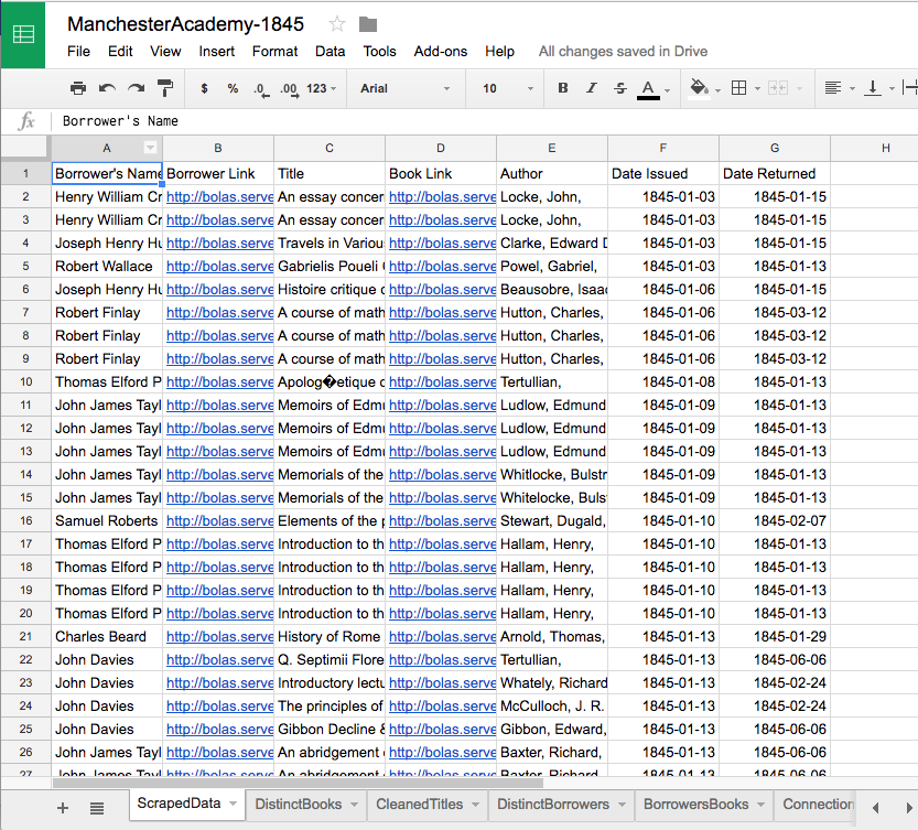
(I renamed this sheet from the generic “Sheet1” to the more descriptive “ScrapedData.” That’s the sheet title I’ll use in the instructions below.)
Generally speaking, I’d say it’s a good idea to leave this page just as it is and make any changes in new sheets—that way, you can always step back to your original data, if need be. In this case, though, there’s a little quirk in the borrower’s names as they got pulled in from Dissenting Academies Online that’s worth fixing before we go any farther.
Before we even begin…
For some reason, there’s an invisible non-breaking space character before the last names of the borrowers in Dissenting Academies Online’s loan search results page. In Sheets, it just looks a little odd. But the reason to get rid of it now is that, if we don’t, our visualization at Kumu will have labels like “Charles Beard.” Gross.
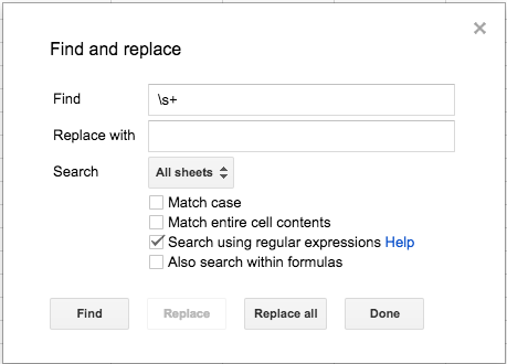
We can fix this with a special find-and-replace operation in Google Sheets. Select Edit > Find and replace… and select “Search using regular expressions.” In the “Find” box, type \s+ (this means “more than one white-space character”). In the “Replace” box, type a single space (using the space bar), then click “Replace all.” We’ll talk a little bit more about regular expressions in a bit…
Okay, now we can start…
Keeping in mind that we need a list of entities to include in our graph, our first step is to come up with one list of the distinct books in our results and another list of the distinct borrowers in the lending records. That is, we need to remove the duplicates.
Getting distinct titles
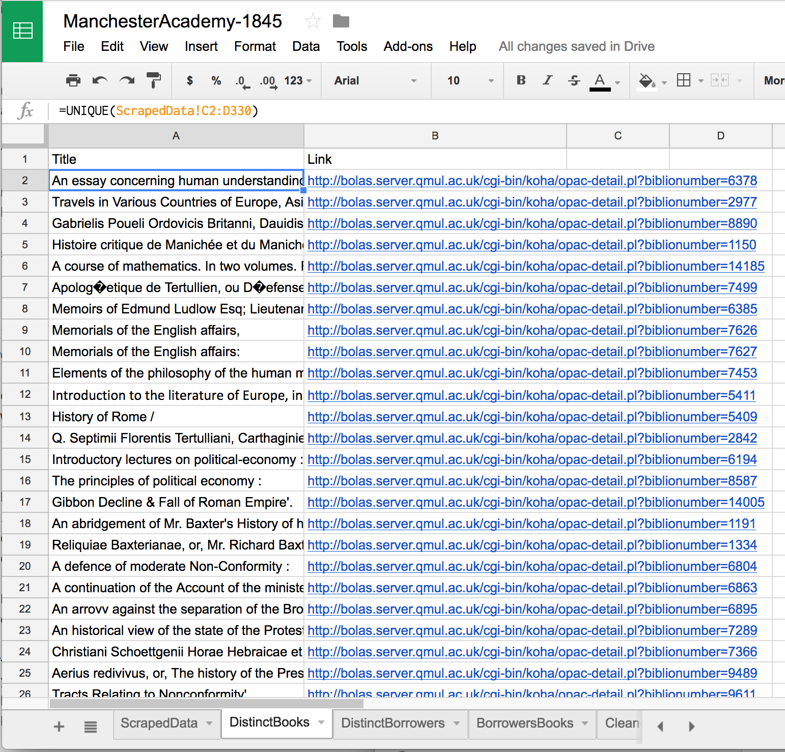
Let’s start by creating a new sheet in our workbook. Call it “DistinctBooks.” Provide column headings “Title” and “Link” in cells A1 and B1. Then, in cell A2, type =UNIQUE(ScrapedData!C2:D330). This function pulls in the contents of the corresponding cells in our ScrapedData sheet, and filters out the duplicates. When you hit enter, columns A and B will fill with the information you’ve pulled from ScrapedData.
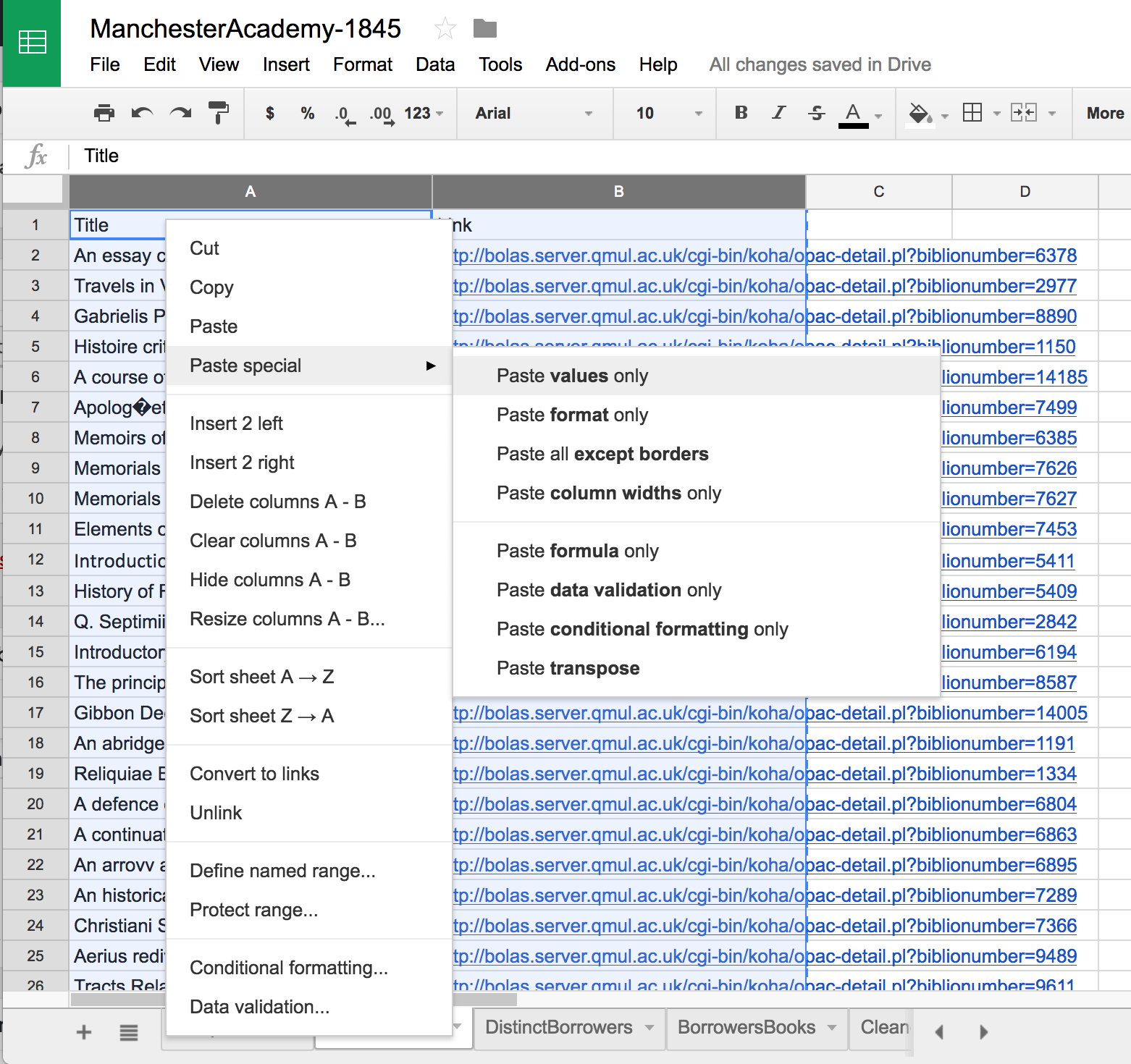
So long as cell A2 contains that formula, the contents of columns A and B will remain dynamic. Let’s make them less volatile by copying columns A and B, then, with those columns still highlighted, right-clicking in cell A1 and pasting just the values (using Paste special > Paste values only). (We’ll do this a lot as we proceed. From here on out I’ll just say “paste the values.”)
At this point, I want to stop for a moment to clean up these titles a little bit—many of them have punctuation at the ends that are artifacts of the MARC records that Dissenting Academies drew on. There are also one or two nasty character encoding problems that bit them on diacritical characters in foreign languages. The second set of problems is small enough that we can clean them by hand, but for the first set of problems, lets revisit Google Sheets’ ability to find and replace text using regular expressions.
Regular expressions allow us to search not just for particular strings of characters, but for generic patterns of characters. Regular expressions can be confusing, so I’m just going to walk you through how to solve this particular problem. (If you want to learn more, there’s a solid, quick primer here. If you find yourself really wanting to learn how to use regular expressions—and they can be immensely useful—you might want to check out the interactive regular expressions tester at Regexr.com.)
If we think generically about the problems we see in these title fields, we’ll find that the issue is that there can be any of several “bad” characters at the ends of the title fields. The set of “bad” characters is actually manageably small, though; in addition to extra spaces, we see commas, semicolons, colons, single quotes, pipes, equals signs, periods, and forward slashes. That’s really not so bad.
[Update: Re-reading this post before publishing it, it occurs to me that there’s a simpler, more elegant solution than the one I outline below: [\W]*$ would remove zero or more non-word characters at the end of the string. That would take care of all the problems I identified in the next paragraph as well as any I might have missed. Plus, it’s easier to type.]
Insert a new column in your DistinctBooks page between the Title column and the Link column. Copy the contents of column A into this new column B and change the title of column B to “Cleaned Titles.” Now highlight the Cleaned Titles column and select Edit > Find and replace. Be sure that your search is set to “Specific range” and that you’re searching column B (you should be), then click the box by “Search using regular expressions.” In the “Find” box, enter this text: [,;:'|=\.\/\s]*$ and leave “Replace with” blank.
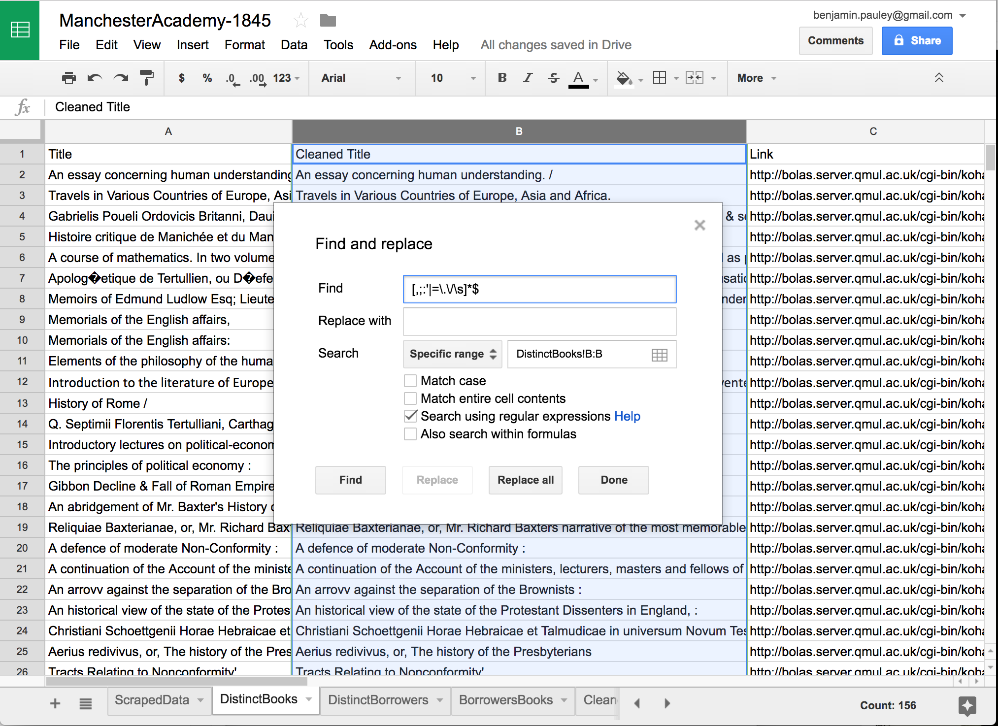
When you click “Replace all,” the contents of column B will change, and those “bad” characters will disappear from the ends of all your titles. Without going too much further into regular expressions, I’ll just note that we told Google Sheets to look for any of the characters within square brackets (a couple of these characters—period and forward slash—have special meanings in regular expressions, so we have to “escape” those characters by placing a back slash in front of them; the \s is, similarly, a special representation of a whitespace character.) The asterisk after our bracketed set means “zero or more” of the characters, which allows us to catch cases where we might have two spaces, a comma and a space, etc. Finally, the dollar sign at the end of the regular expression means “at the end of the string.” So our regular expression is looking at the end of the title field for zero or more of the “bad” characters we identified and then replacing them… with nothing. Problem solved.
We still have the problem of the strange “�” characters that appear here and there. (This is some sort of character encoding problem that probably happened as Dissenting Academies brought data in from another source. It happens.) A search of our Cleaned Title column shows that that character appears five times, which is a small enough number that we could just clean them up one at a time. But where’s the fun in that? Four of the five times, it turns out, we get “�e” where we should get “é”. The fifth time, however, we get “i�” where we should get “iæ”. A couple of find-and-replaces later, we can get rid of those errors, too.
Getting distinct borrowers
To get a list of the distinct borrowers in this data set, we can do the same thing for people that we did for books. Create a new sheet, title it “DistinctBorrowers,” then label cell A1 “Borrower Name” and label cell B1 “Borrower Link.” In cell A2, type =UNIQUE(ScrapedData!A2:B330) and we’ll pull in the each of the unique names and links from the corresponding cells in our ScrapedData sheet.
I want to do one other thing with these names that will draw on our work with XPaths in Part I. If we look at an individual borrowing record at Dissenting Academies Online, we’ll see that the borrower’s name is given as a link:
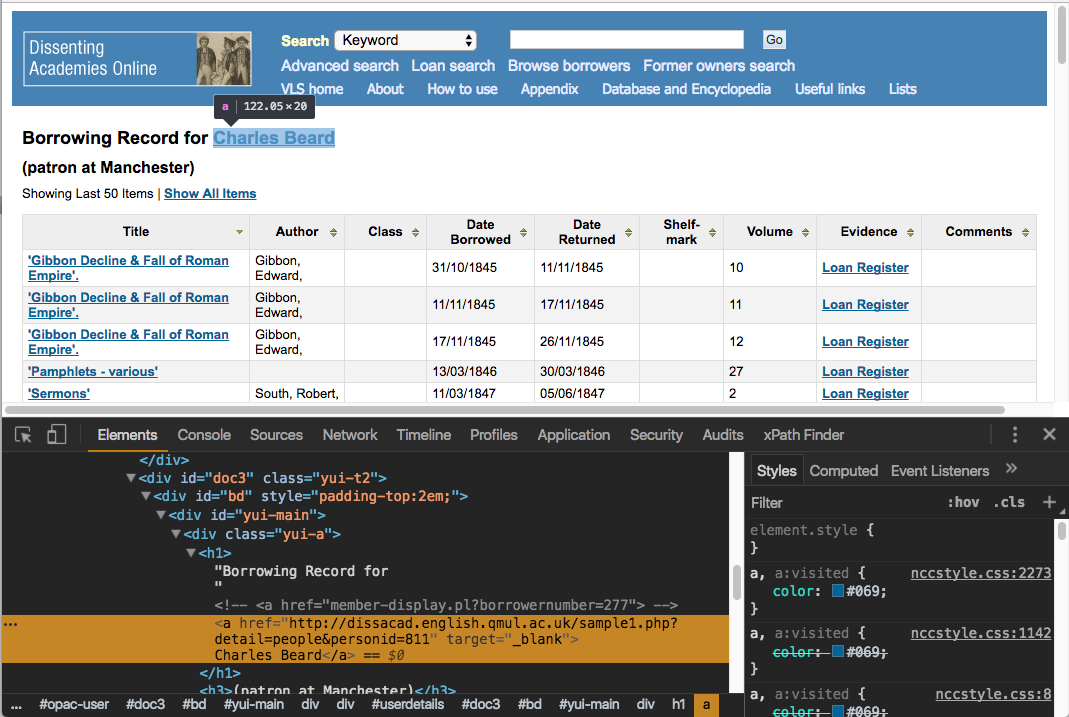
Following that link takes us to the encyclopedia entry for that borrower in the broader Dissenting Academies Online project. Those entries can provide some interesting information, so it would be nice to be able to refer users of our visualization to it directly.
The IMPORTXML() function Google Sheets allows us to pull in data from a web source directly, without having to use a tool like Scraper. We just need to have a URL (which we have in column B) and an XPath (which we know how to figure out). Label cell C1 “Biographical Record” then type in cell C2: =IMPORTXML(B2,"//h1/a/@href"). When you hit enter, you’ll see a message that says “Loading” for a moment, and then a link will appear. You can then copy the formula from C2 and paste it into cells C3 through C22, then watch as Sheets pulls in the rest of your links.
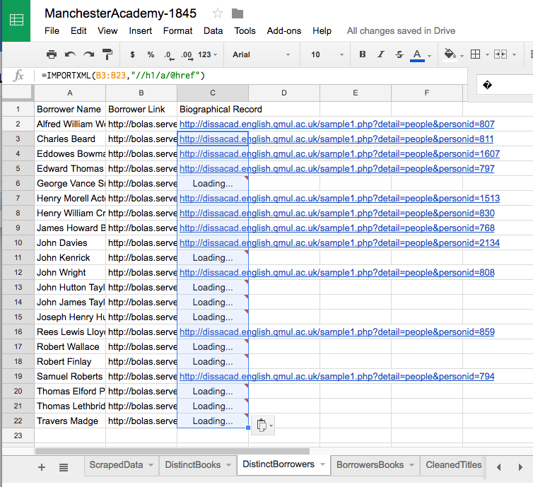
(I like to then copy all those links and paste the values over the formulas so Google Sheets doesn’t try to fetch the URLs again later, for any reason.)
Who borrowed what? (Making the “Connections” list)
So far, we’ve been working on assembling a list of books and a list of people. We’re going to come back to those in a bit to compile them all into a single sheet for importing into Kumu. For now, though, I want to turn to the other question we need to address to get ready to bring all this into Kumu: the connections between borrowers and books.
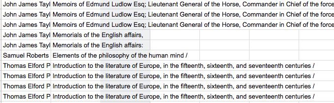
Create a new sheet and call it “BorrowersBooks,” then label column A “from” and column B “to” (those are the labels Kumu will be looking for). [Update: It looks like Kumu is insisting on lower-case “from” and “to.” I don’t think that was the case before, but it seems to be the case now.] In cell A2, type: =ARRAYFORMULA(ScrapedData!A2:A328), which will pull in the contents of column A from our ScrapedData sheet. In cell B2, type: =ARRAYFORMULA(ScrapedData!C2:C328) to pull in the titles. (Keep in mind, these are the “dirty” titles from ScrapedData, not the cleaned-up versions we created a few steps back. We’ll get to that in a minute.)
Now we’ve recreated the connections between borrowers and books from ScrapedData (you could have accomplished the same thing by simply copying and pasting the contents of those columns, actually). Notice, though, that many of these rows are duplicates, as borrowers checked out the same books multiple times:
I’m generally not a fan of duplicate lines. We could just eliminate them by using UNIQUE(), but I don’t want to just throw away information about how many times people borrowed books. So let’s get a count first and then eliminate our duplicates.
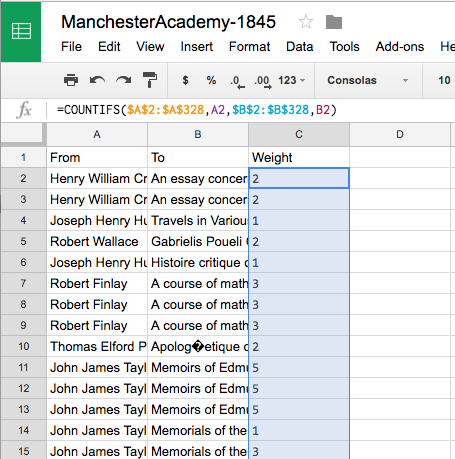
Label column C “weight”, then, in cell C2, type: =COUNTIFS($A$2:$A$328,A2,$B$2:$B$328,B2). (That searches the range A2:A328 for the value in A2, and also searches the range B2:B328 for the value in B2 and returns the number of times that both of those conditions turn out to be true. We have to put the dollar signs before the column and row numbers because we’re going to paste this formula down the rest of column C. If we didn’t use the dollar signs, our range would shift down a row each time, becoming A3:A329, A4:A330, etc.) Hit enter and you should get “2” as a result. Now copy and paste the formula from C2 into C3 through C328 to get the rest of your counts. Once you have your results, it would be a good idea to copy them and paste the values over top of the formulas.
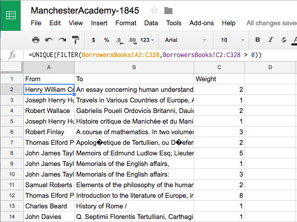
Now to get rid of the duplicates and clean up our titles. Create a new sheet (I promise, the end is near) and call it “Connections.” Label column A “From”, column B “To”, and column C “Weight.” Then, in cell A2, type: =UNIQUE(FILTER(BorrowersBooks!A2:C328,BorrowersBooks!C2:C328 > 0)). This formula uses UNIQUE() to get rid of duplicates. The other bit in there is meant to filter out a couple of odd cases where there is a borrower’s name but no title. (In some instances, Dissenting Academies has someone borrowing a book on a certain day, but apparently we don’t know what the book was—there’s no title, no link, no nothing.) The FILTER() function is looking at the range of cells A2:C328 in the BorrowersBooks sheet and checking to be sure that the number in column C is greater than zero. Only after a row passes that test does it then get handed over to the UNIQUE() function.
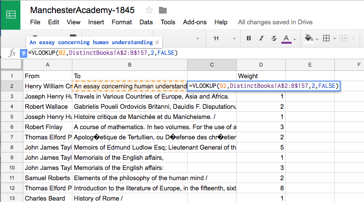
Now let’s clean up those titles. I debated doing this at a much earlier stage—making it so we’d have had the cleaned titles to draw on in some of our earlier steps—but I really wanted you to experience the VLOOKUP() function, which can be really useful. Copy all the data on the sheet and then paste the values over it. Next, insert a column between columns B and C (your old column C will become column D). Then, in your new cell C2, type: =VLOOKUP(B2,DistinctBooks!A$2:B$157,2,FALSE). This looks for the value of B2 in the first column of the range A2:B157 on the sheet DistinctBooks (i.e., column A, our “dirty” titles). When it finds that value in column A, it returns the value in the second column in the range (i.e., column B, our “clean” titles). (The “False” flag says that column A of DistinctBooks is not sorted, so VLOOKUP() shouldn’t just stop at the first thing that looks like a match.)
Copy that formula and paste it into the other cells in your new column, and you’ll get “clean” versions of all of your titles. Then copy those clean titles, paste the values over the “dirty” titles in column B, and delete column C, leaving you once again with “From,” “To,” and “Weight,” only this time with cleaned titles.
This case—searching a long string of text to get a different long string of text—is sort of a strange use for VLOOKUP() can come in very handy when you have a table of values where the value of one column can serve as a reliable index for identifying the row. This comes up a lot when you download data from a web site—there will often be some kind of unique identifier for a record that you’ll want to be able to look up.
Now we’ve got a list of unique connections between borrowers and (cleaned) book titles, along with weights reflecting how many times that borrower borrowed that title. Copy all of this information and then paste the values so we don’t have to worry about losing any of our references to other sheets or cells.
That takes care of the “Connections” sheet that Kumu needs. Now, back to the “Elements” sheet.
The “Elements Sheet” (we’re almost done with Google Sheets, I swear)
We really already have pretty much everything we need for the “Elements” sheet on our DistinctBooks and DistinctBorrowers sheets. We just need to combine that information in one place and add a column that notes which rows are books and which rows are borrowers, and (this part is optional) add another column with any descriptive text we want to provide.
Create one last sheet and call it “Elements.” Label column A “label,” column B “type,” and column C “description.” In cell A2, type: =ARRAYFORMULA(DistinctBorrowers!A2:A22) (or just copy and paste those cells from the DistinctBorrowers sheet). Enter “Borrower” in cell B2, then copy and paste that value into cells B3 through B22.
[Update: Apparently, I had forgotten how I had done this when writing the tutorial. To get a line break, we need the HTML tag for a line break rather than simply a newline character.] For our descriptions, I want to show links back to Dissenting Academies Online, so we’re going to construct the contents of those links using the CONCATENATE() function to assemble the HTML that we want to upload to Kumu. This looks tricky, but is pretty simple. In cell C2, type: =CONCATENATE("<a href='",DistinctBorrowers!B2,"'>Borrowing Record</a><br /><a href='",DistinctBorrowers!C2,"'>Biographical Record</a>"). Let’s go through it in steps. CONCATENATE() just pastes together whatever strings of text you give it. In this case, we’re providing some of those strings ourselves in quotation marks, and some as references to the contents of other cells. So we start with the beginning of an HTML anchor tag: <a href='. Then we pull in the URL from cell B2 of DistinctBorrowers to use as the value of the href attribute. Then we finish the beginning of the anchor tag, provide the text that we want to display for the link, and close the anchor tag: '>Borrowing Record</a>. The rest of our CONCATENATE() formula is just adding a line break (<br />) and doing the very same thing for the link to the biographical entry at Dissenting Academies Online. Copy and paste that formula down for the rest of our borrowers.
[Update: I realize I forgot to finish the Elements sheet]
We now have a list of people’s names, an indication that they are “Borrowers,” and two links back to the data at Dissenting Academies Online. But “Borrowers” are only one of the two kinds of “Elements” we need. We also need “Books.”
Below the last borrower (in A23), type =ARRAYFORMULA(DistinctBooks!B2:B157) to pull in the titles of each of our books. In cell B23, type “Book,” then copy and paste that value down to the end of the list of titles. Finally, in cell C23, type =CONCATENATE("<a href='",DistinctBooks!C2,"'>Book Detail</a>"), and copy that formula down to the end of our list of titles.
We now have one sheet with all our “elements”—both Borrowers and Books. Copy all of this information and then paste the values so we don’t have to worry about losing any references to other sheets or cells.
In Part III, we’ll upload this information to Kumu and get to work styling our network graph.